1
Detection
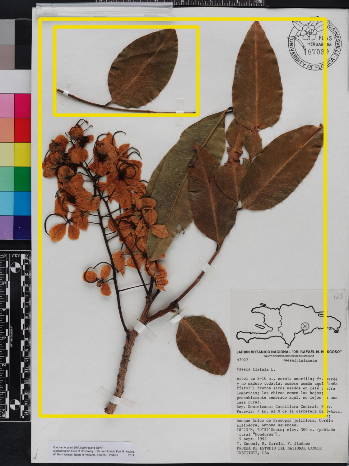
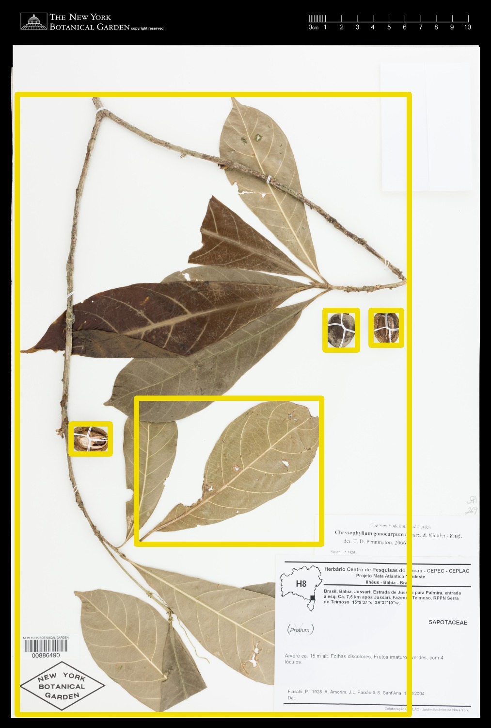
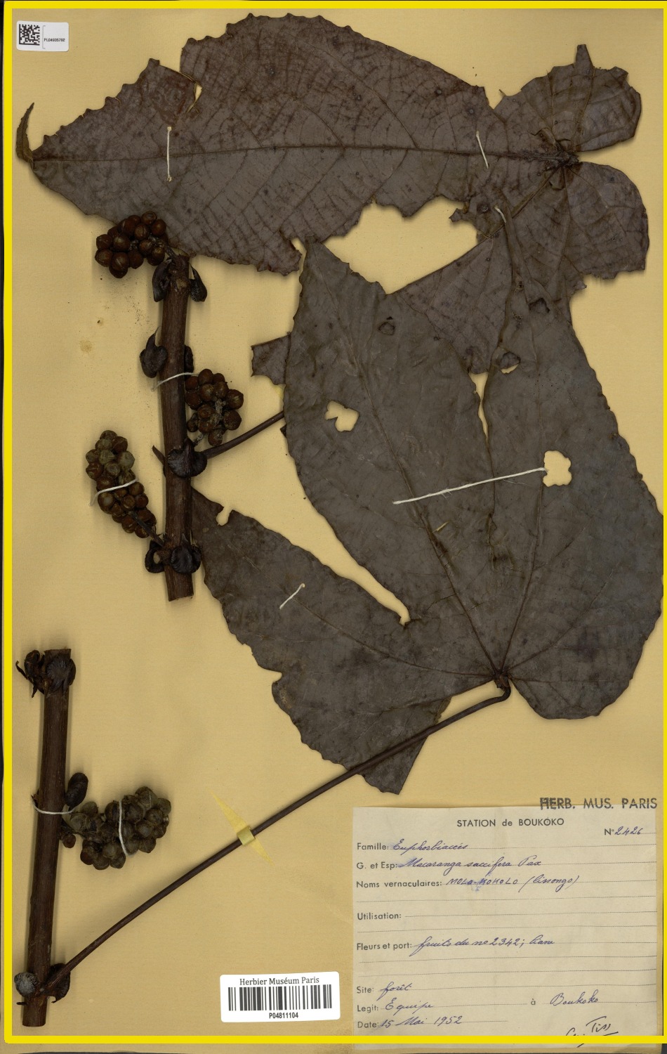
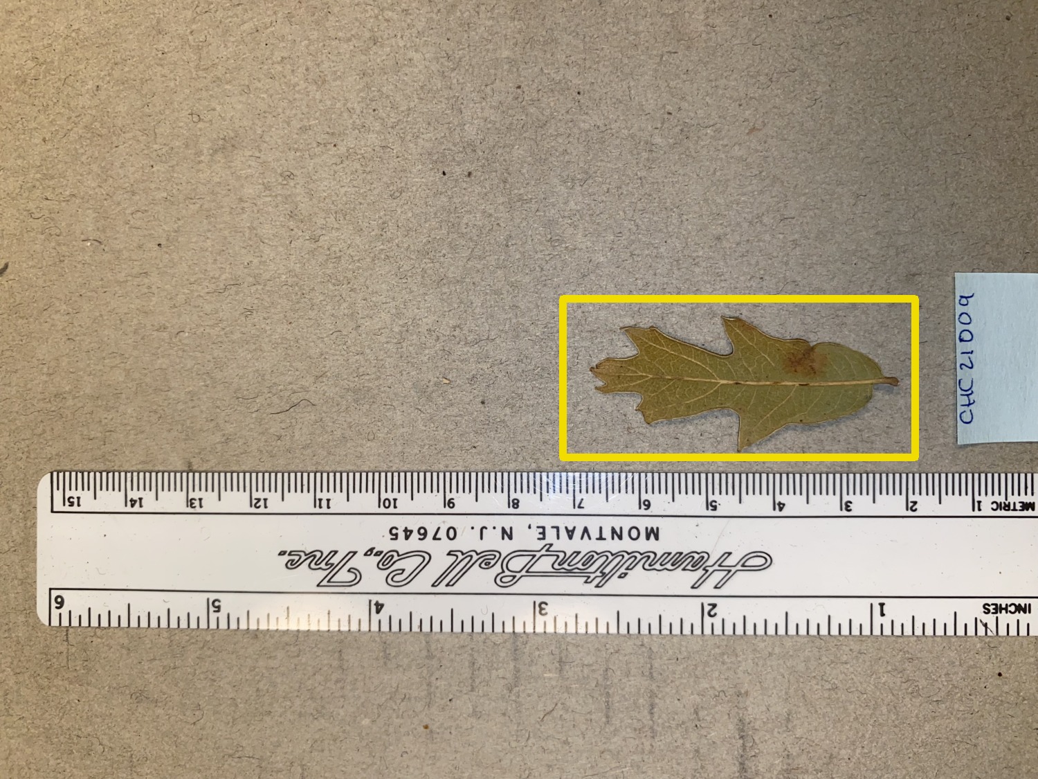
A YOLO detector locates the pressed specimen on each herbarium sheet (yellow box), separating the plant from labels, rulers and colour cards.
From detector boxes to a model that corrects its own training labels. Each step below cleans the previous step's noise; the images are raw QC overlays (no annotations).
A YOLO detector locates the pressed specimen on each herbarium sheet (yellow box), separating the plant from labels, rulers and colour cards.
Each Specimen box prompts SAM3 to produce a first foreground mask. It is a good start but noisy — it bleeds onto the mounting paper and misses thin parts.
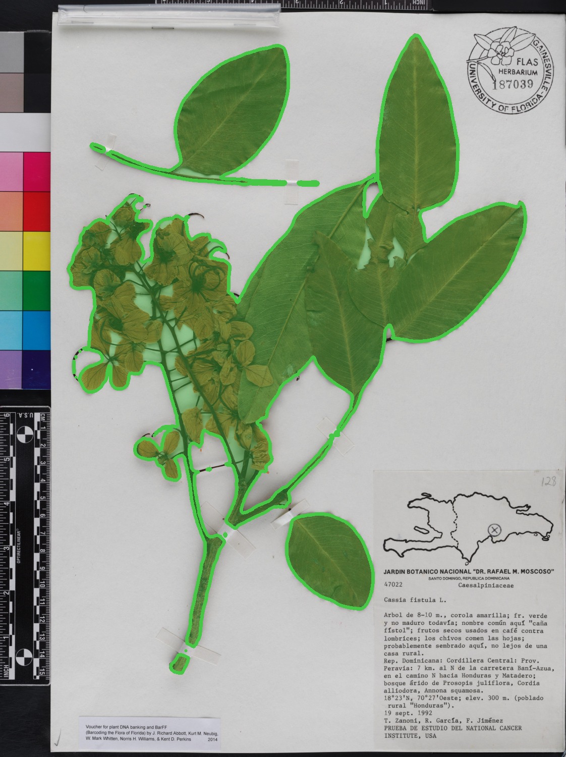
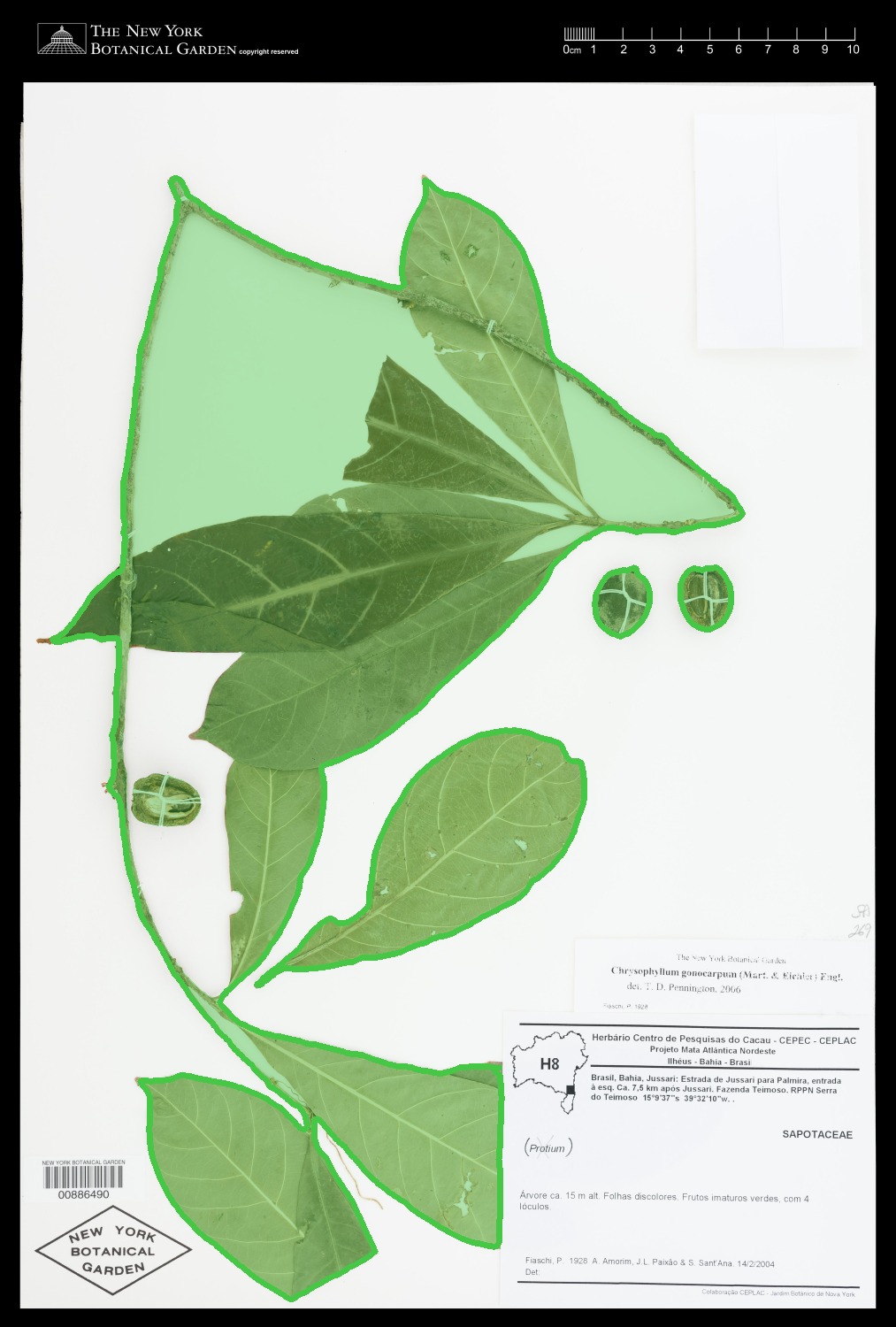
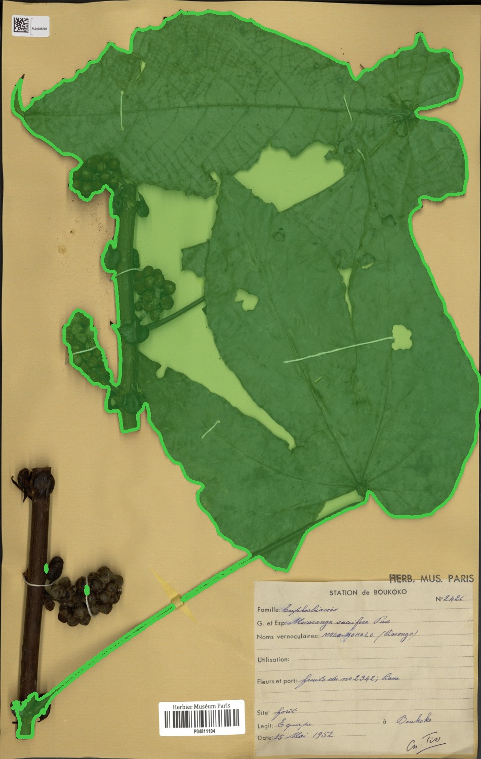
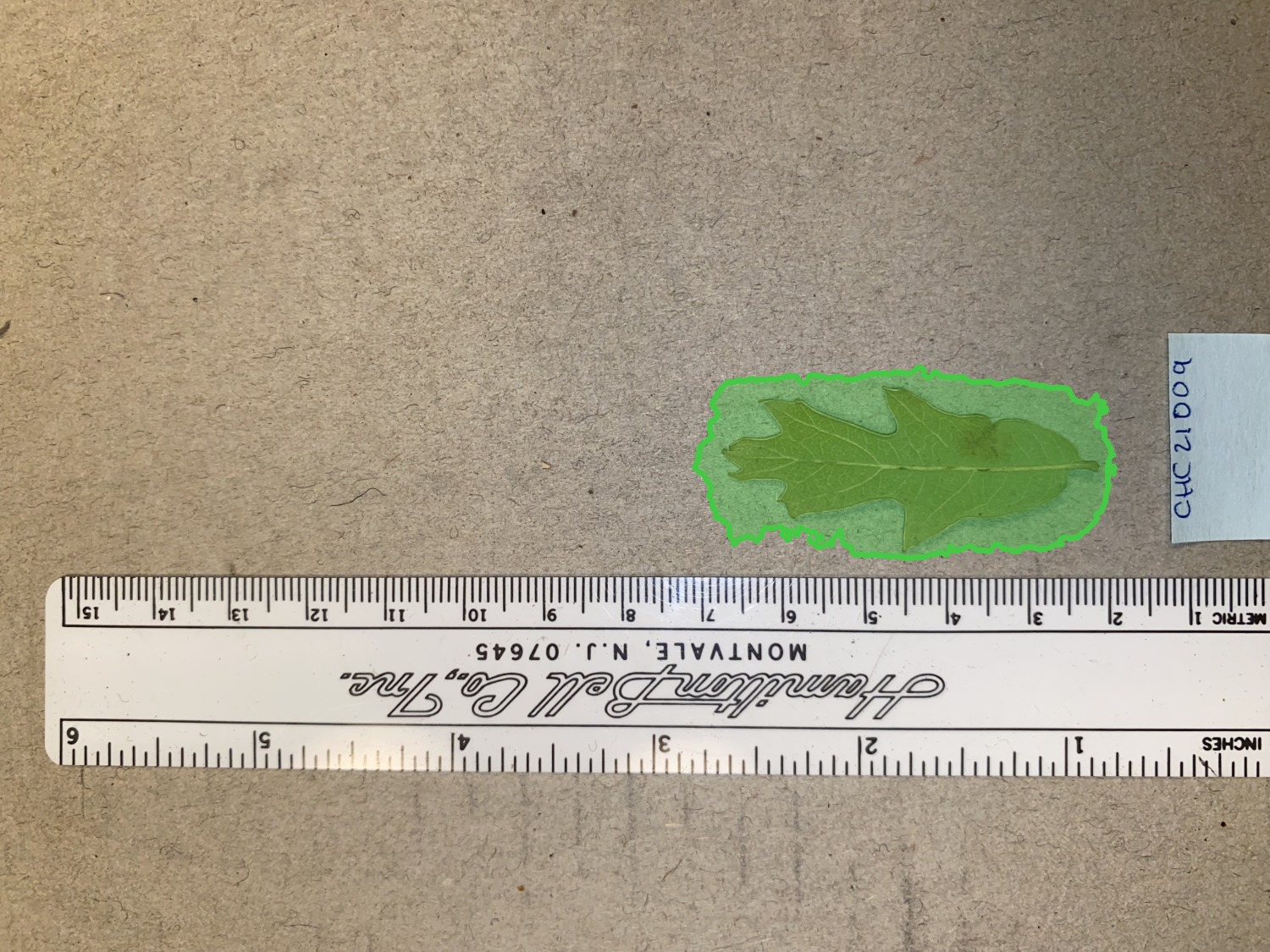
A UNet is trained on the SAM3 masks, then its own predictions replace them. Averaging over the dataset cancels much of SAM3's per-image noise.
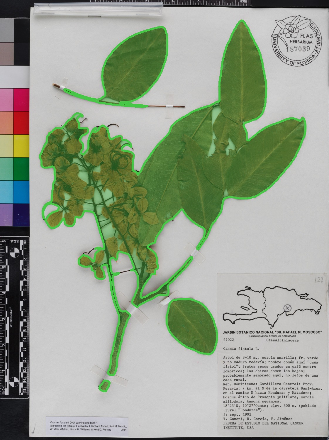
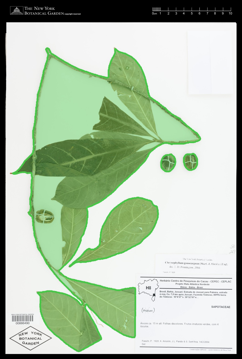
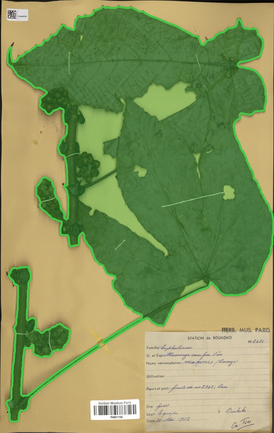
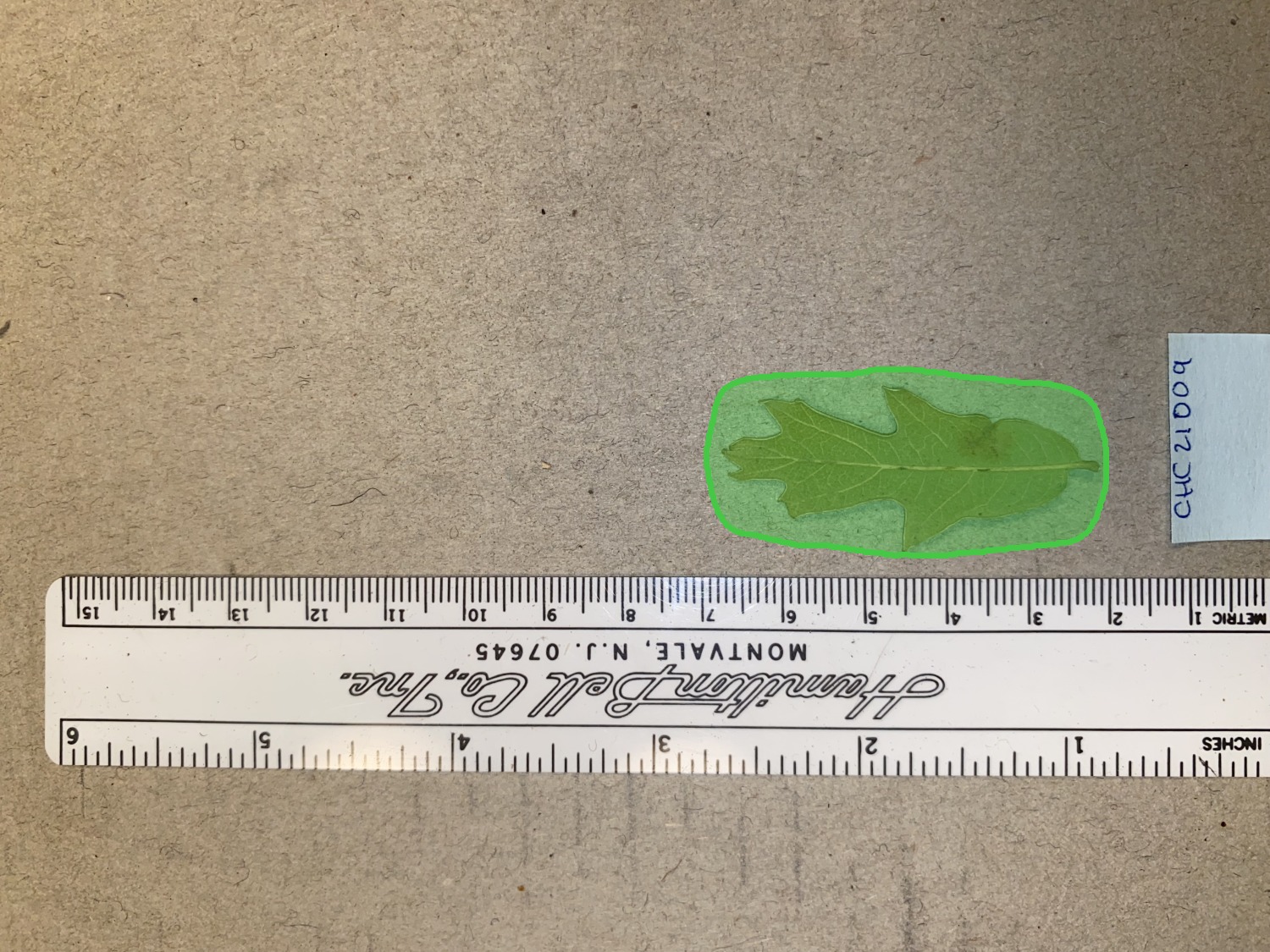
Informed HSV colour segmentation strips the white/yellow mounting paper from inside the mask (shown in red) — interior gaps and the edge halo.
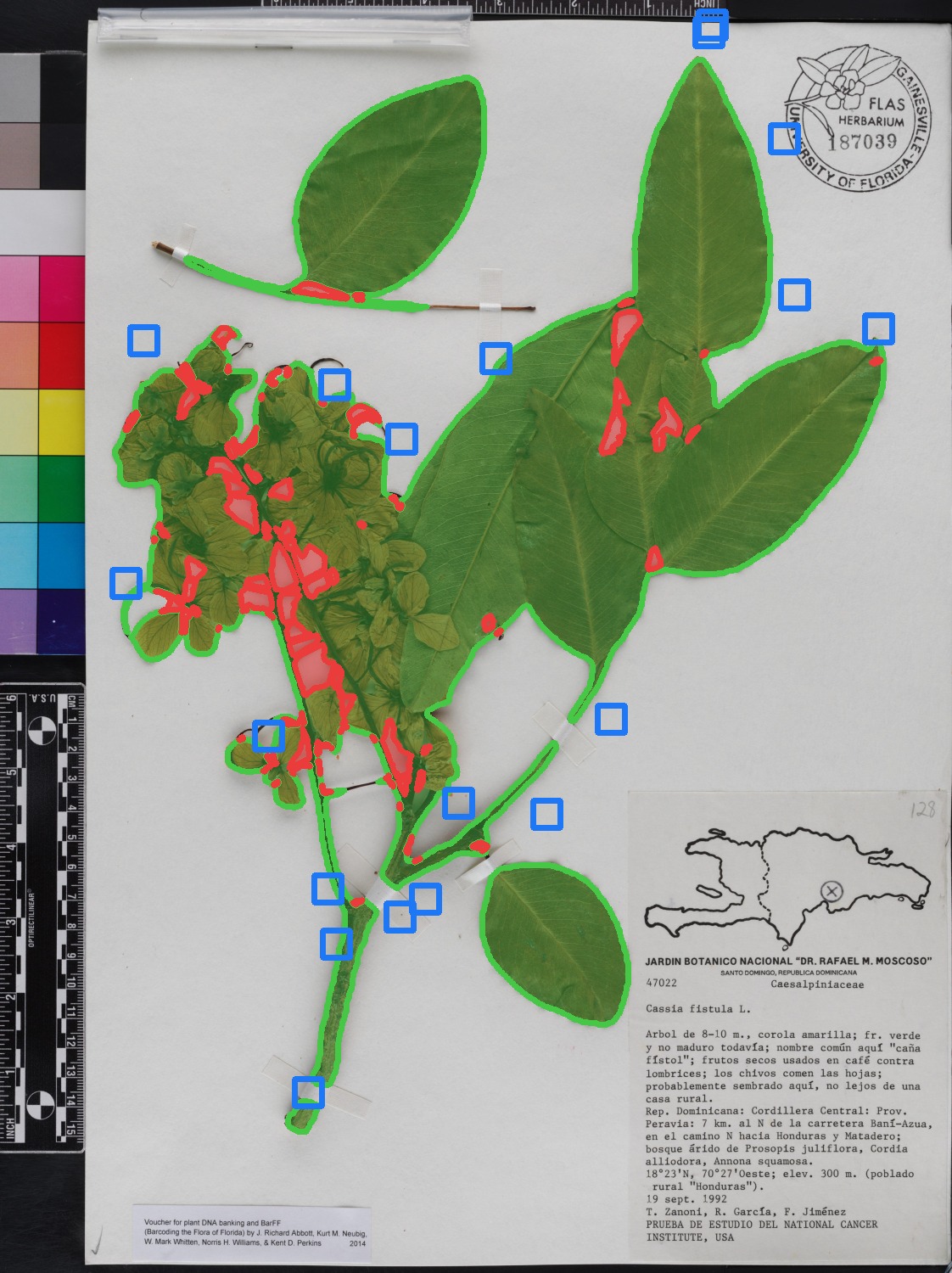
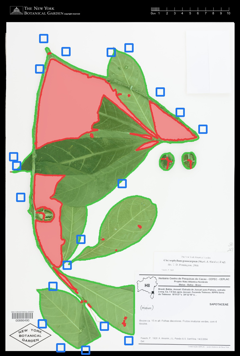
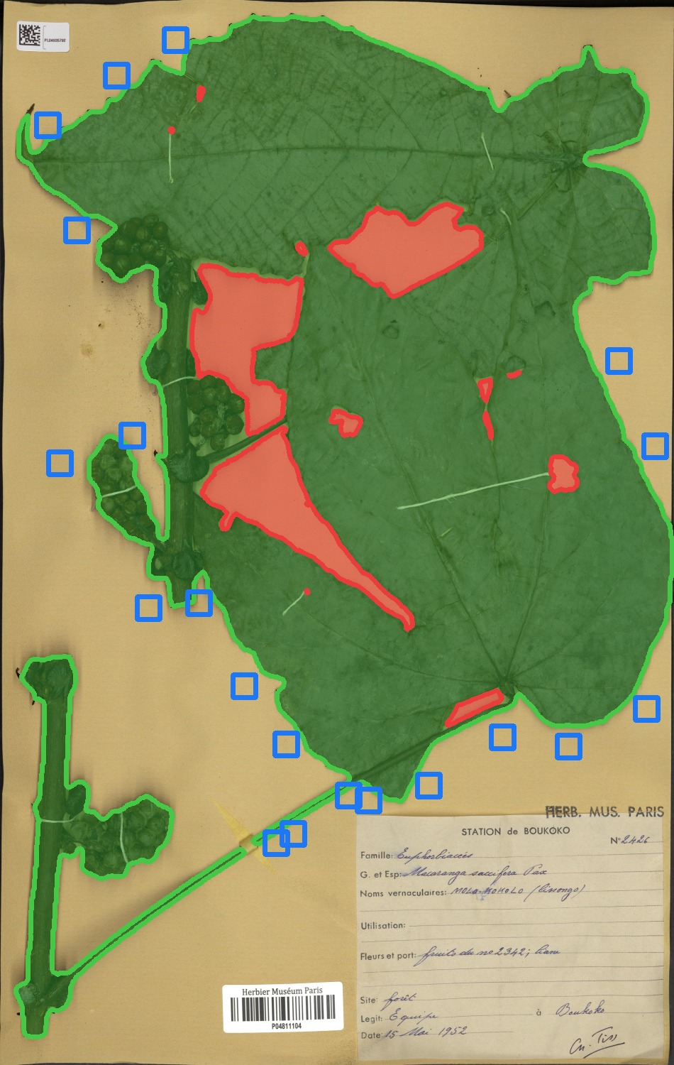
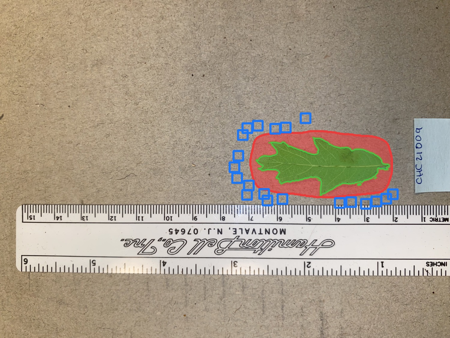
During training the model tracks each image's loss. Labels that stay hard to fit after the model has learned the clean majority are flagged as bad ground truth (red) and down-weighted so they stop poisoning the gradient.
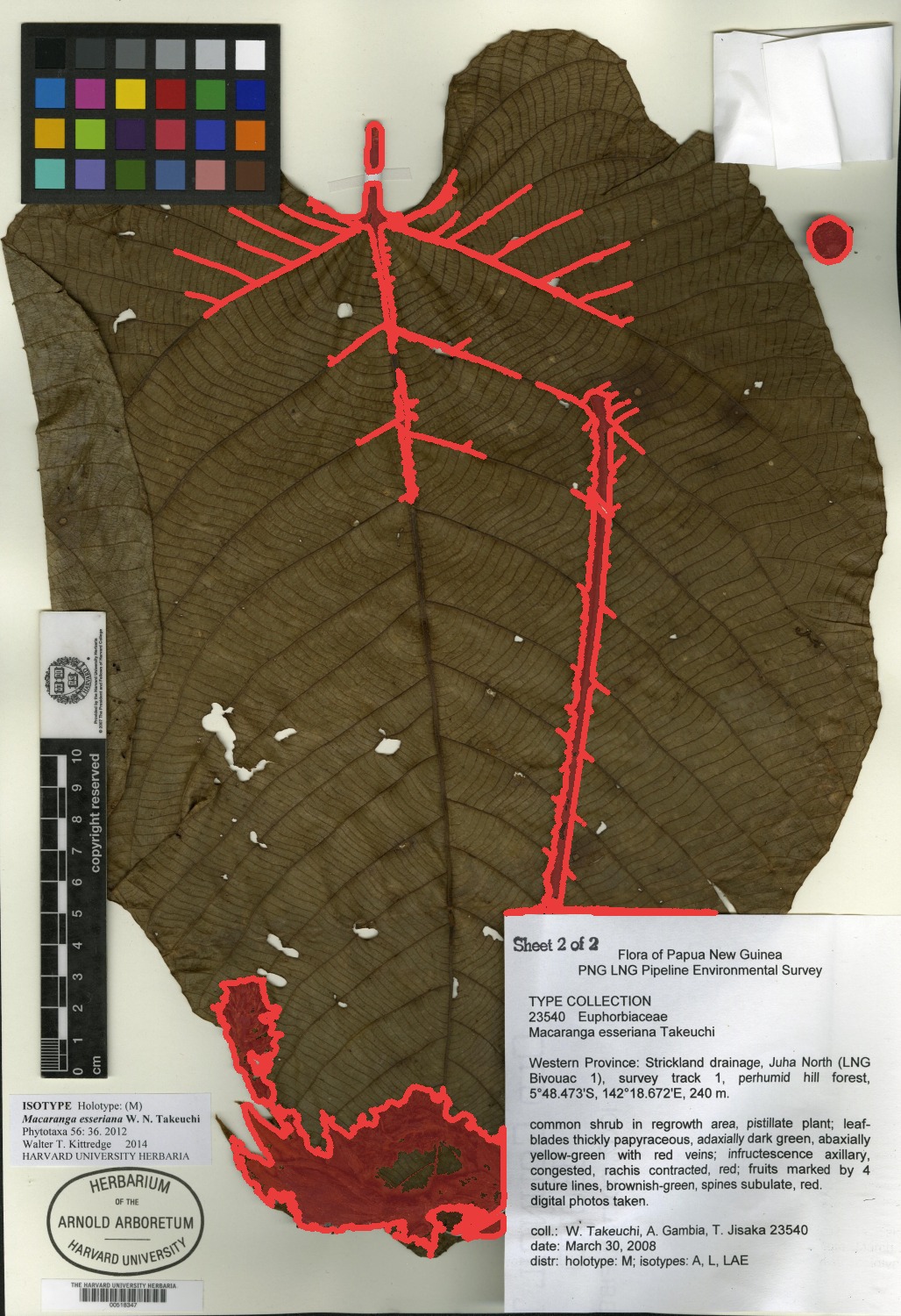
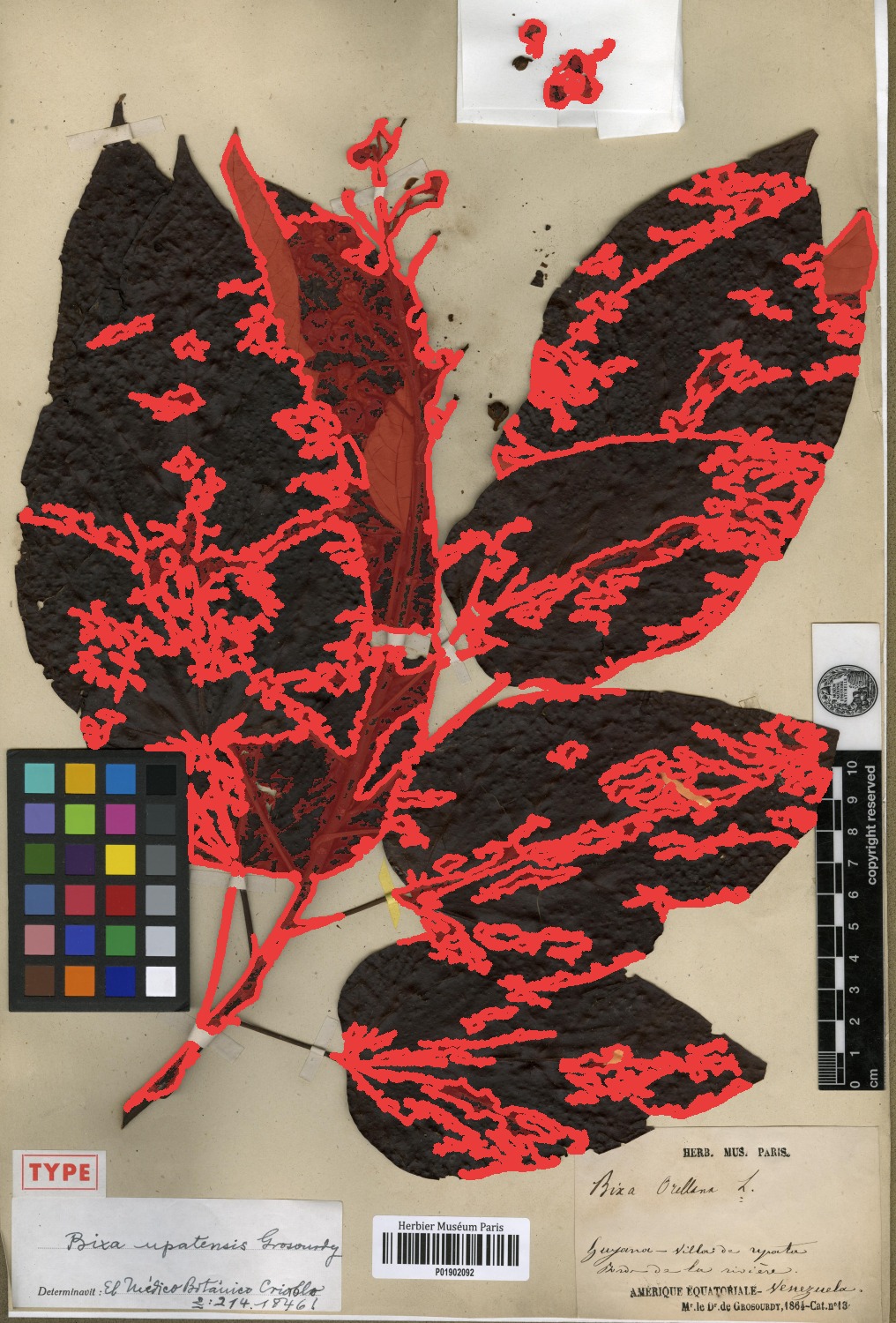
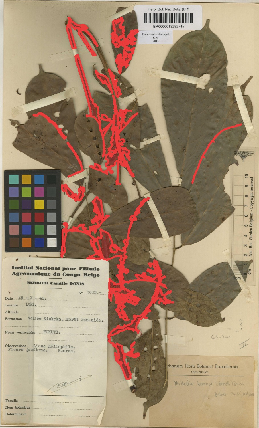
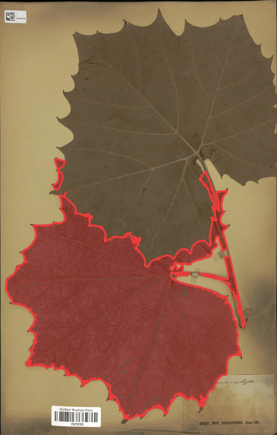
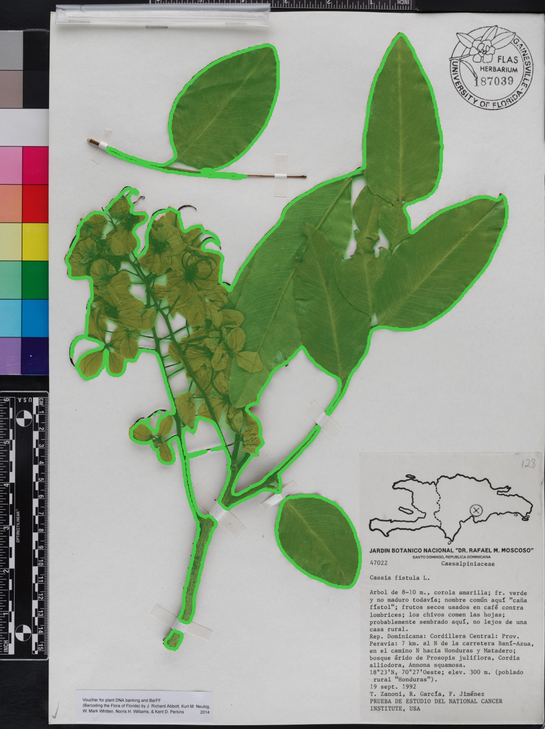
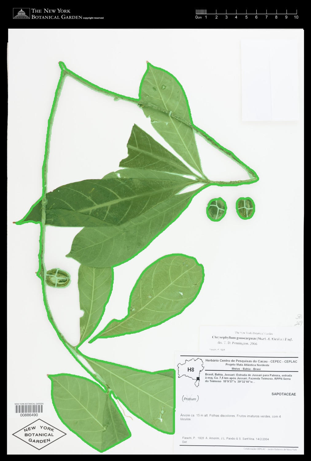
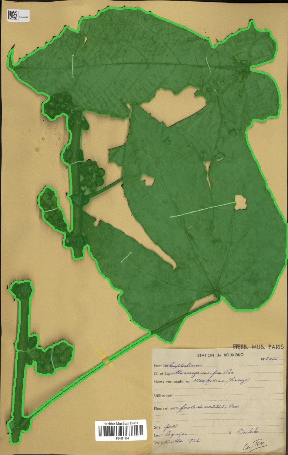
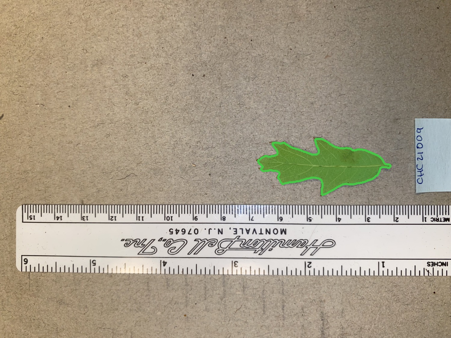
Every few epochs, each flagged image's label is replaced by the model's own prediction (green) — recovering plant material the original mask dropped. The model then trusts its learned prior over the noisy target.
| Original Groundtruth Mask | Self-Relabeled Groundtruth Mask |
|---|---|
| 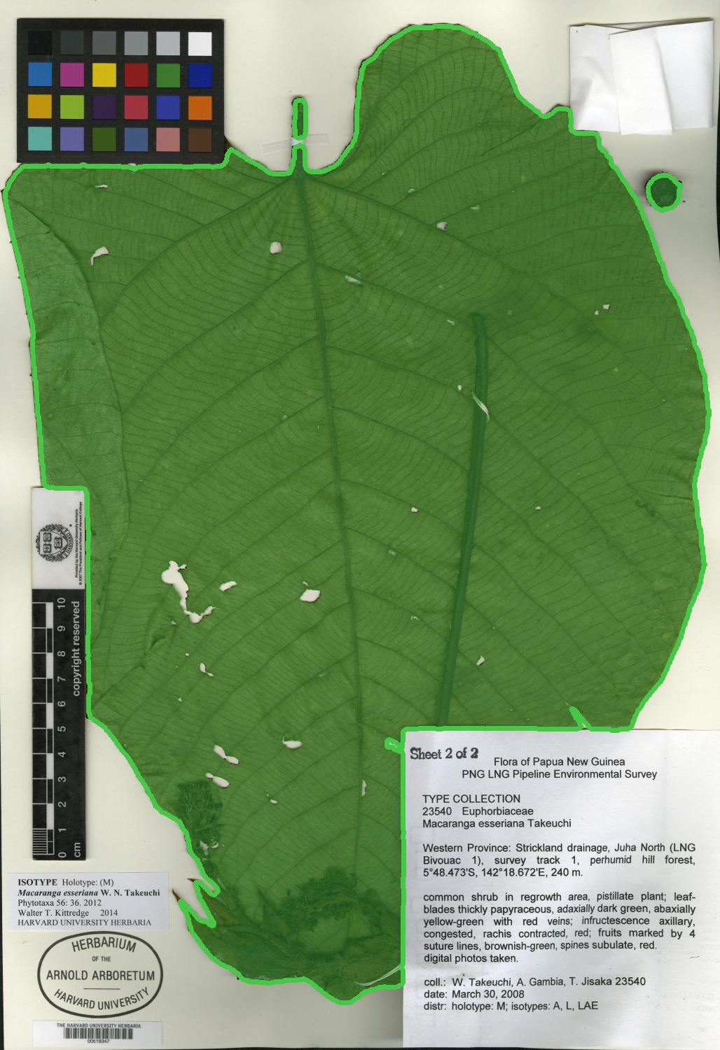 |
| 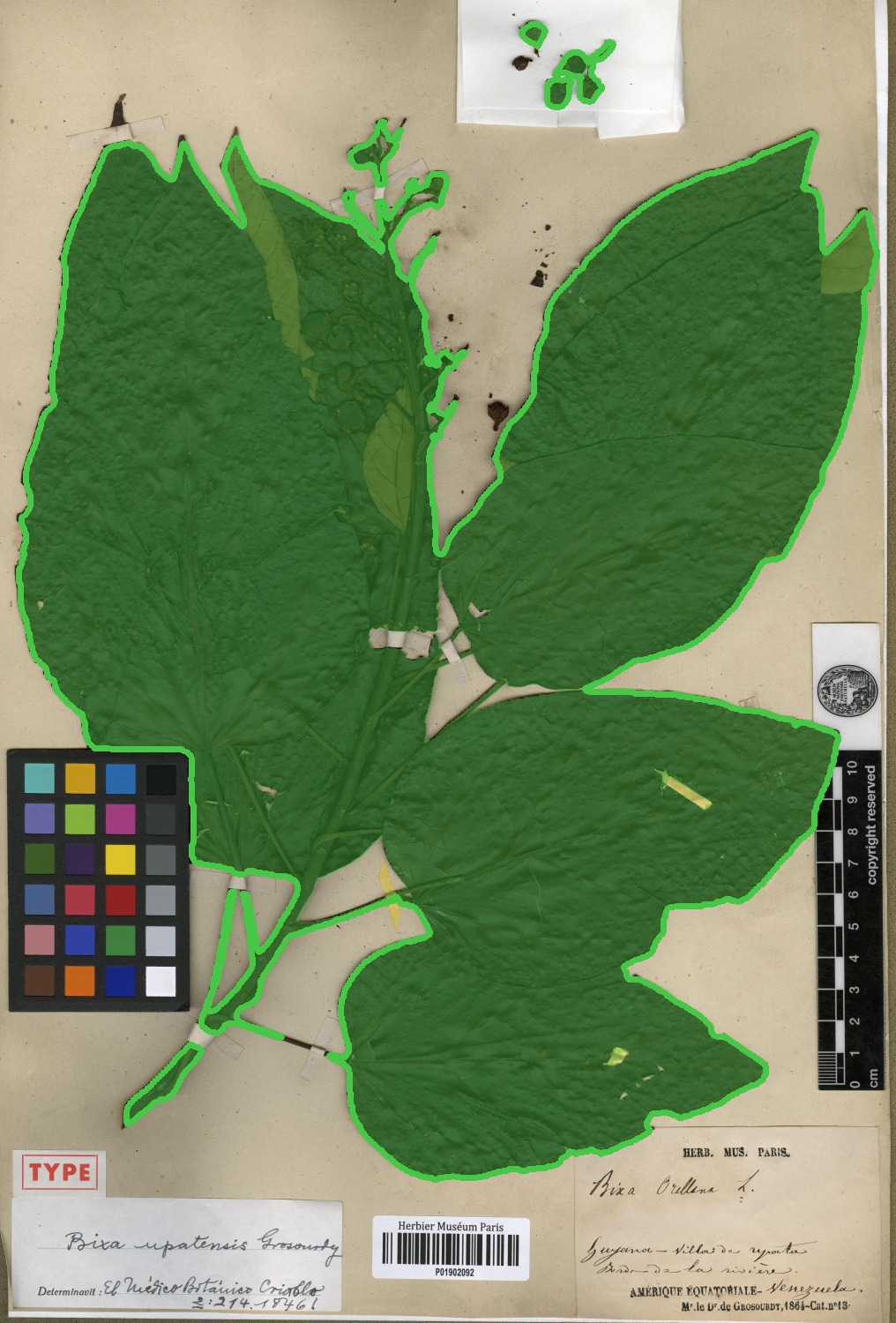 |
| 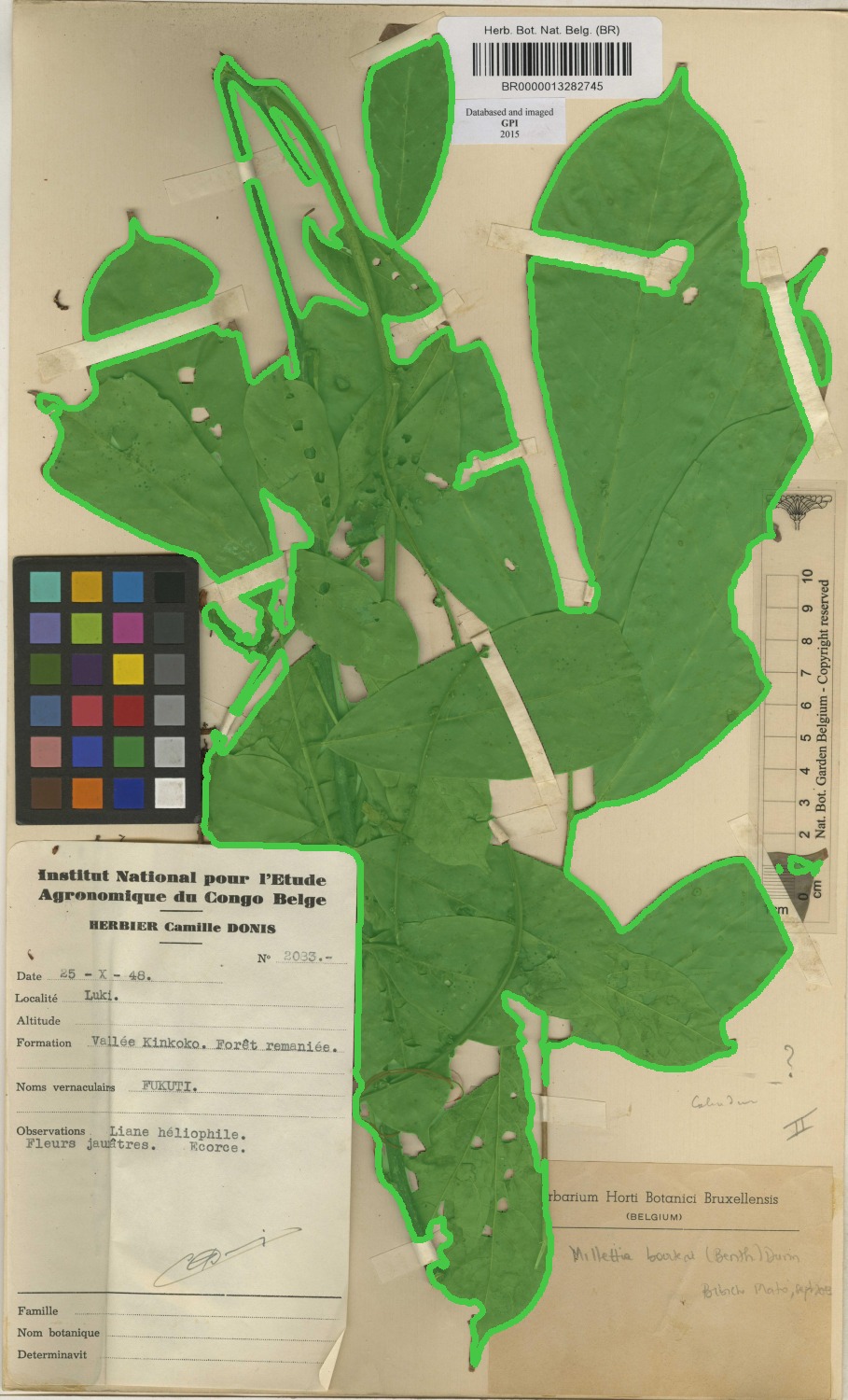 |
| 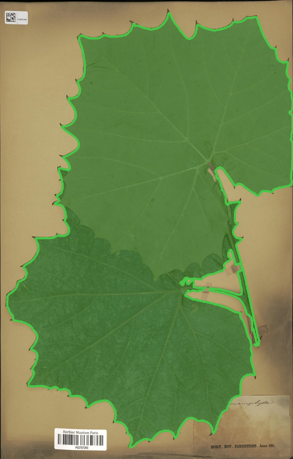 |
The final self-healed model produces clean, paper-free specimen masks — tight to the plant, interior gaps removed, thin structures kept.
The same arc — cheap weak labels to a dense model — on beehive comb frames. A few labelled points per tile, lifted to full segmentation via DINOv2 features and a distilled ResUNet.
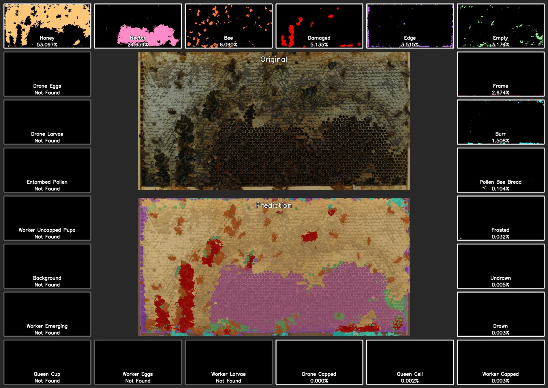
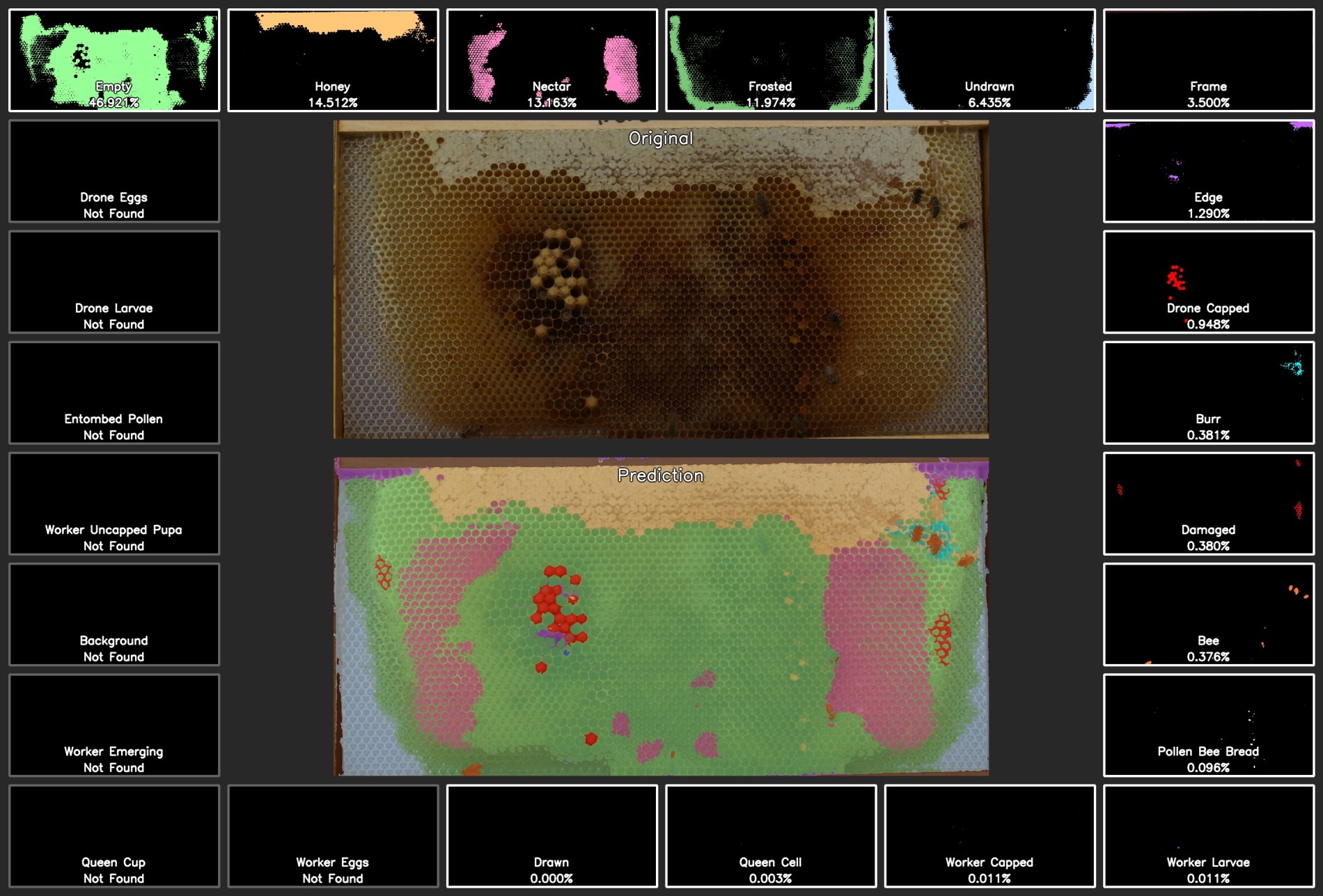
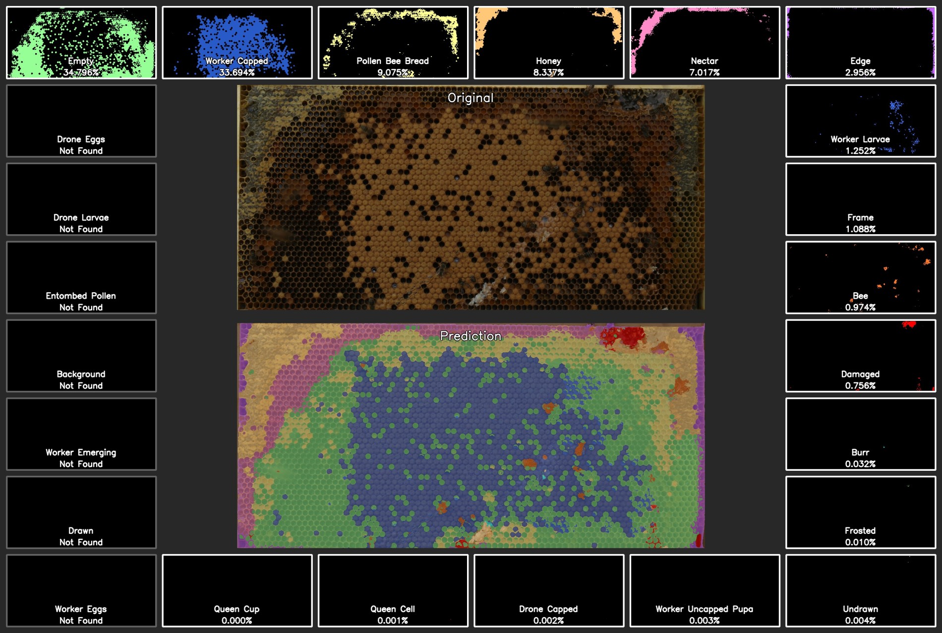
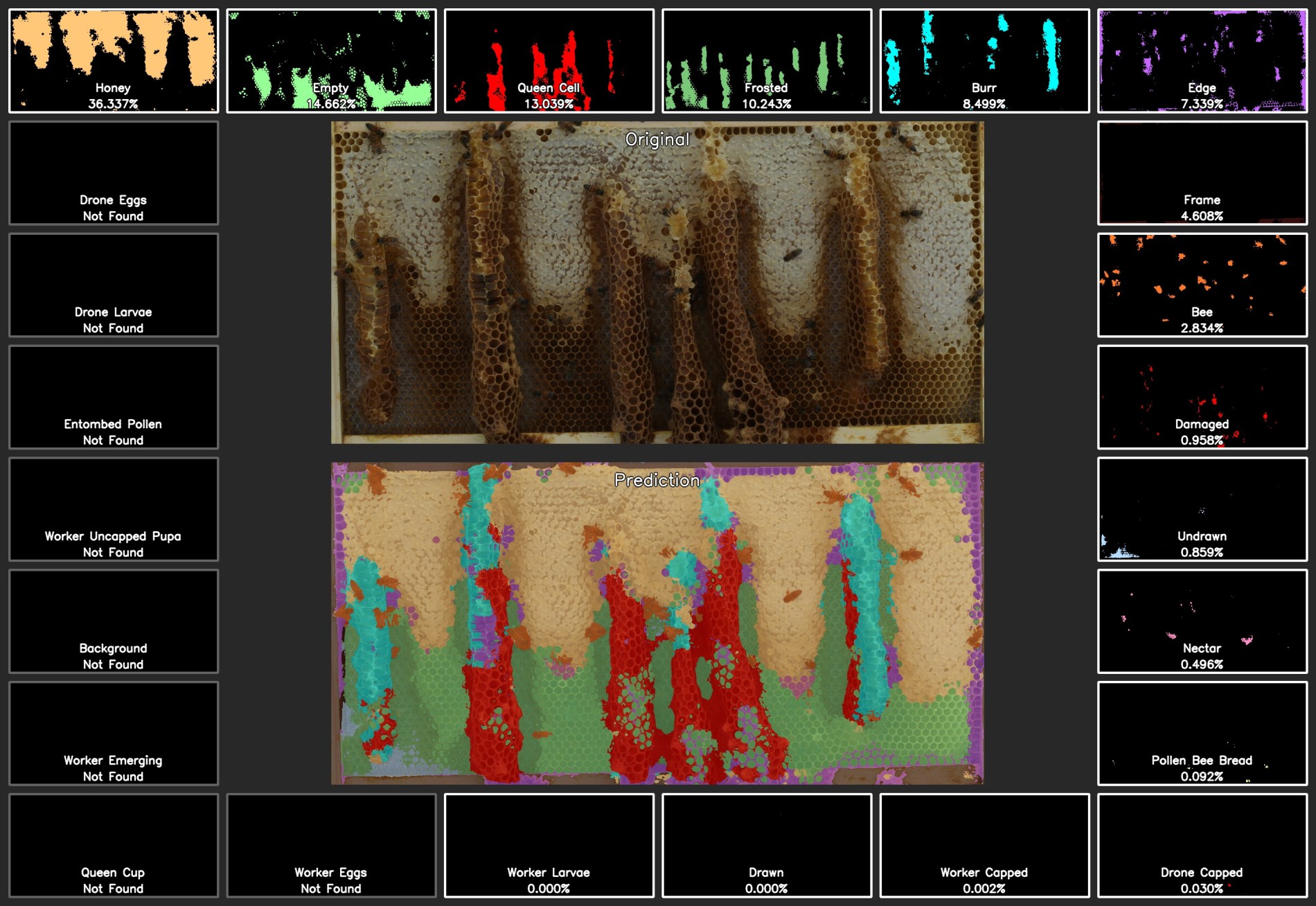
Beekeepers photograph each frame. One frame packs thousands of hexagonal cells whose contents — capped honey, nectar, pollen, brood at many stages, bees, empty comb — are exactly what we need to map.
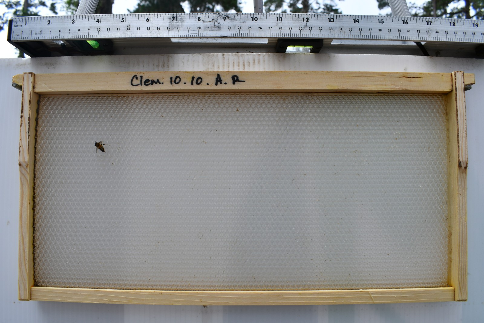
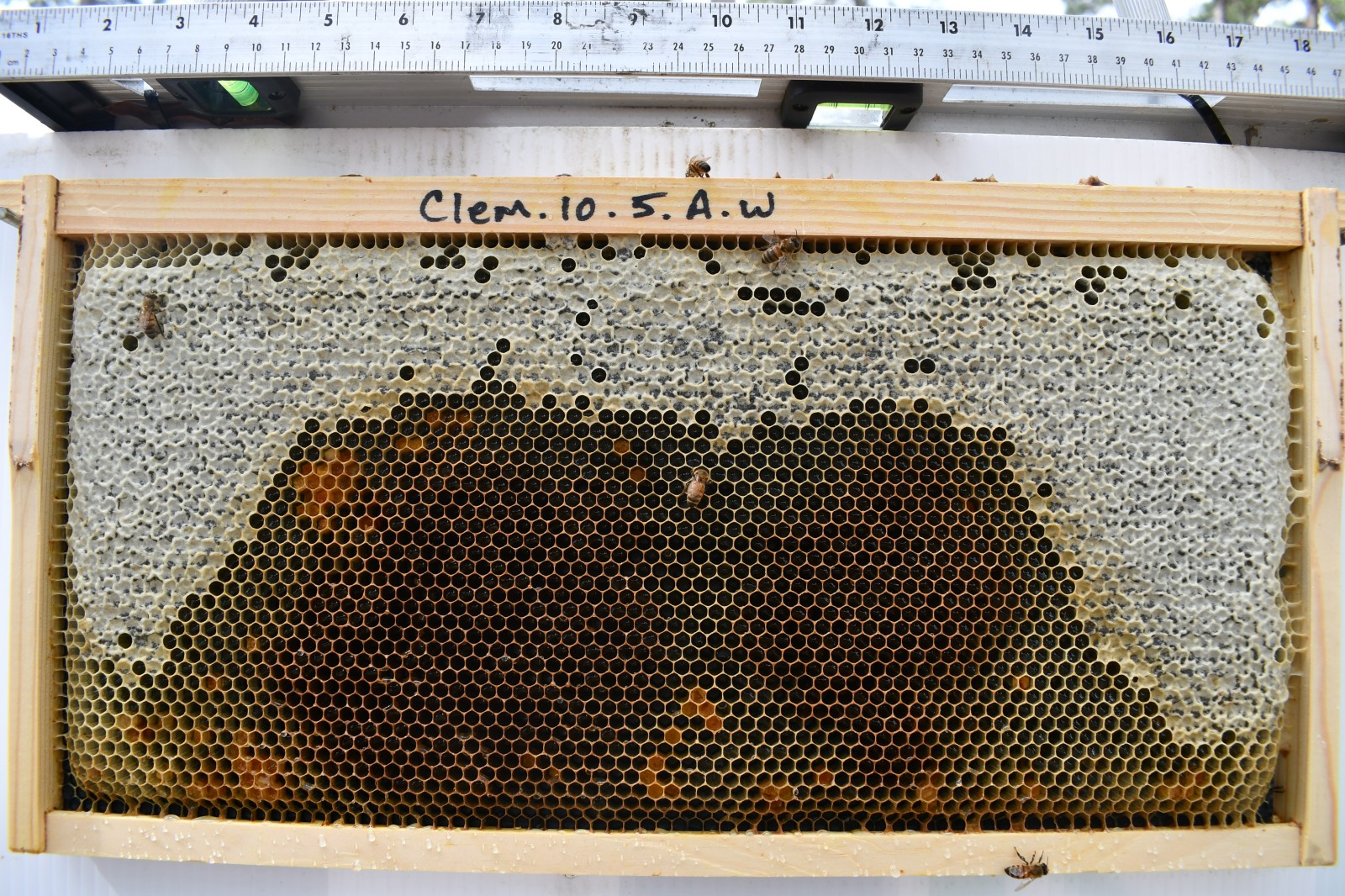
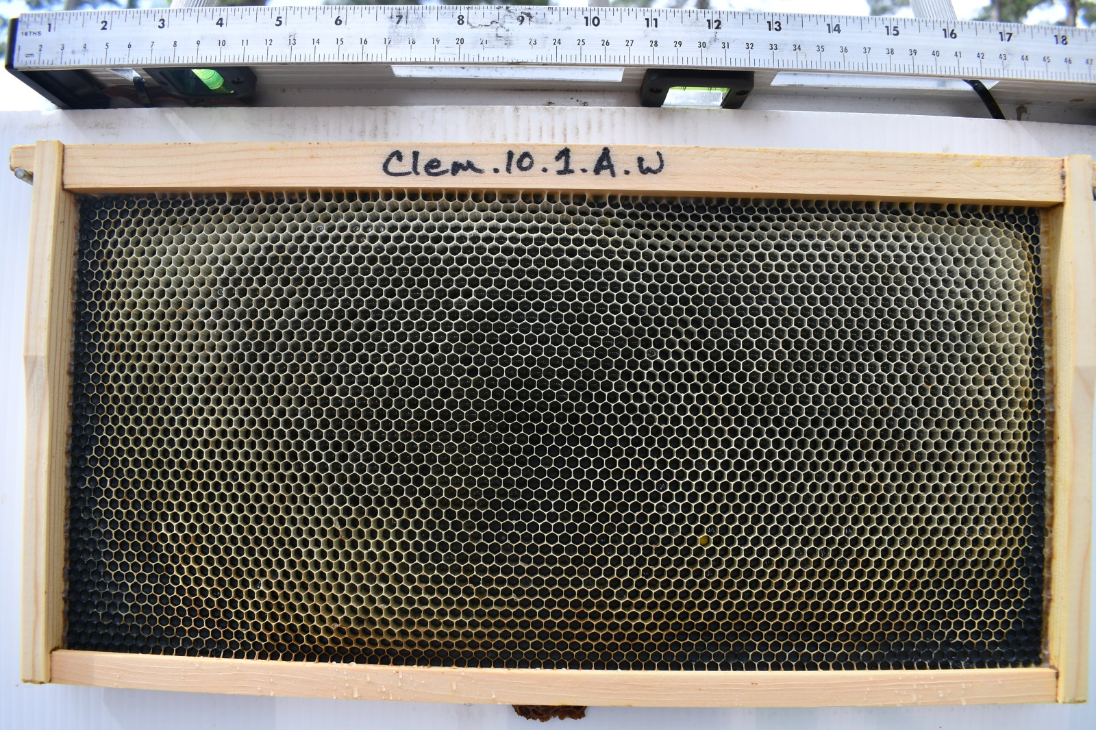
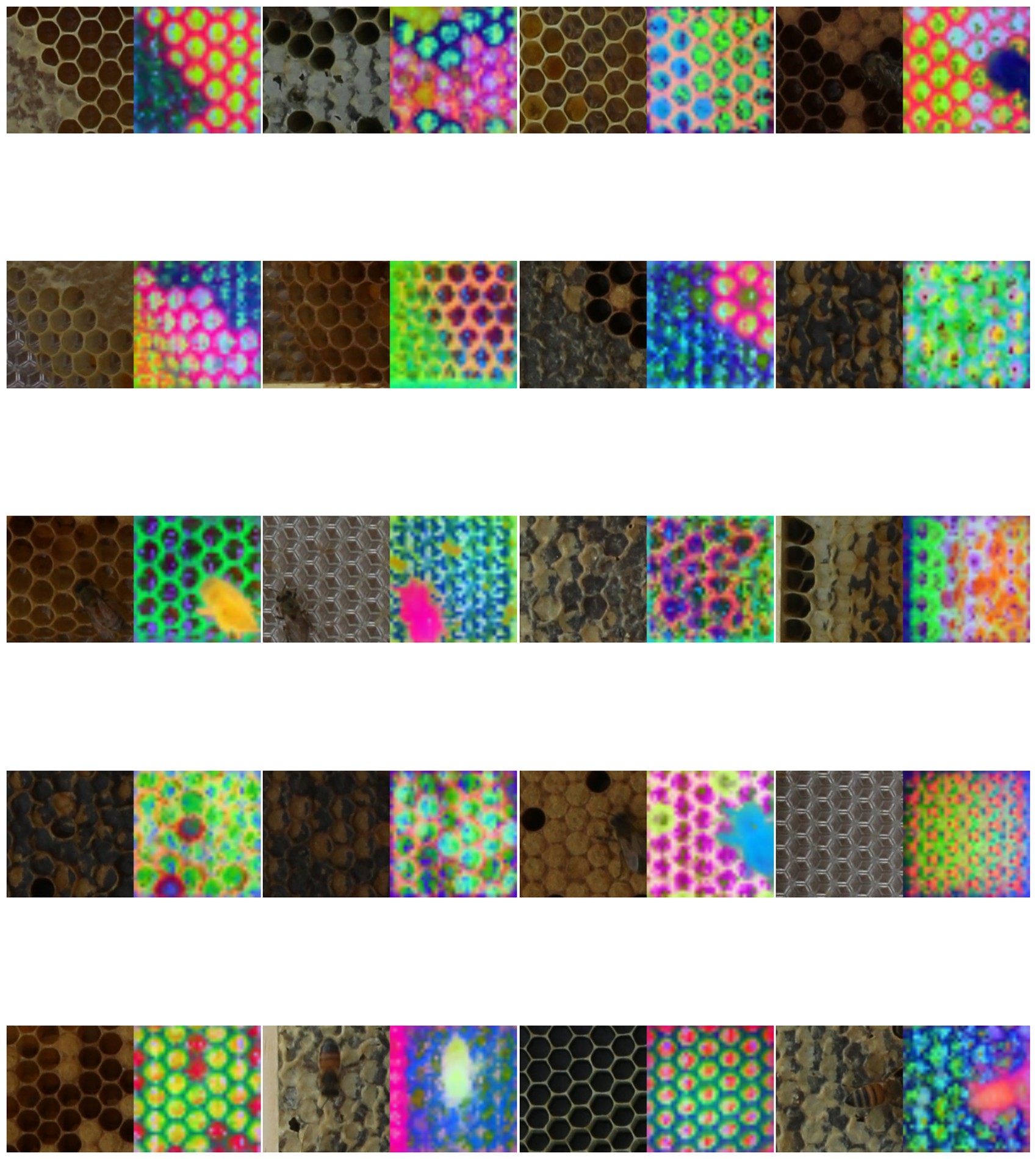
Frames are cut into 224px tiles. Up close the labelling problem is obvious: dozens of cell types blend together with no crisp edges. Hand-tracing every region across 24 classes and thousands of cells, on every frame, is infeasible.
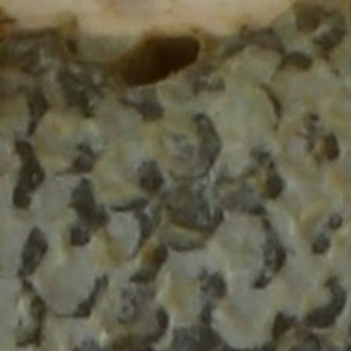
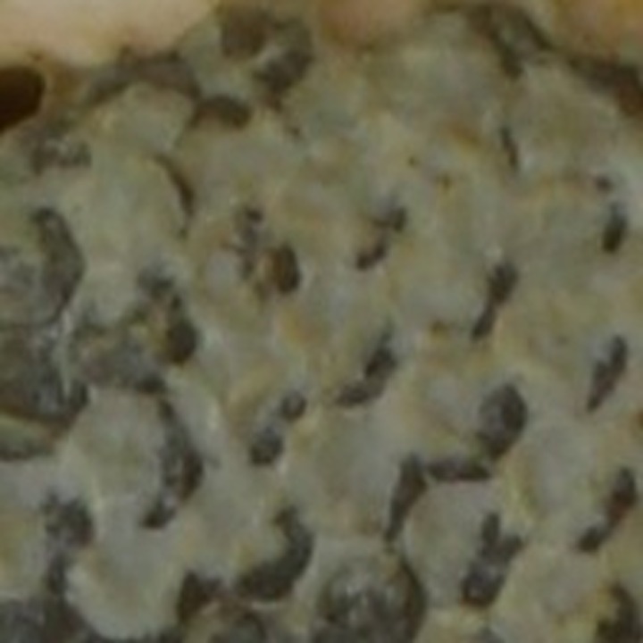
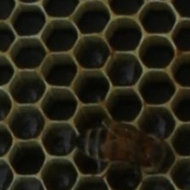
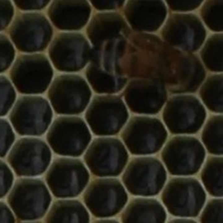
So we don't trace regions — we drop a few labelled points per tile, coloured by class (honey = gold, empty = green, nectar = pink, brood = blue …). A handful of clicks per tile instead of pixel-perfect outlines.
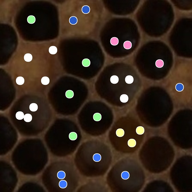
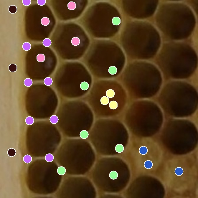
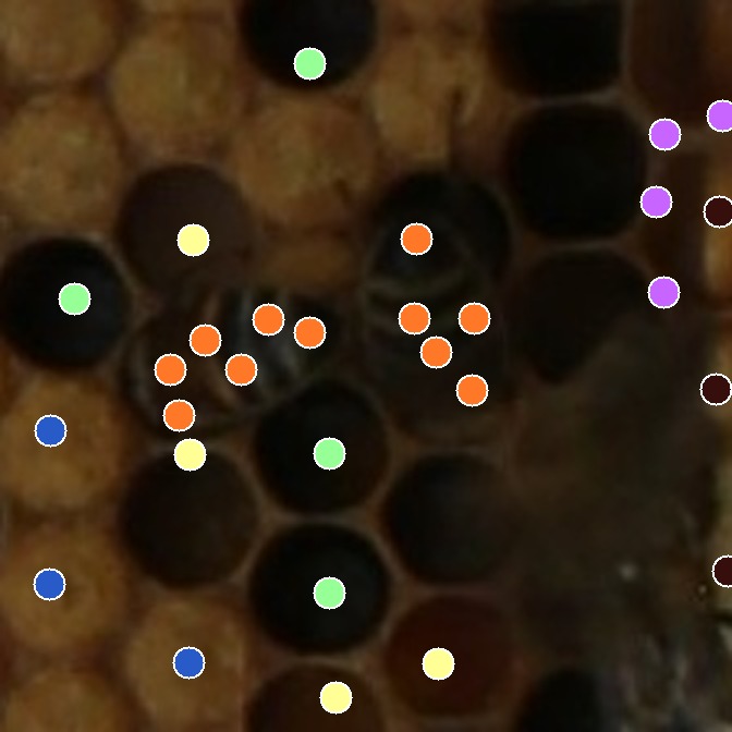
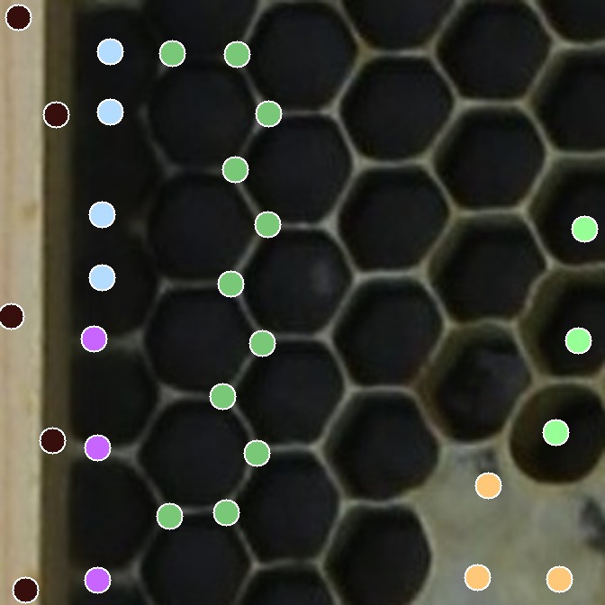
A frozen DINOv2 vision transformer turns each tile into per-patch embeddings. The PCA-coloured features (right) already separate cell types before any training — honey, comb and brood fall into distinct feature clusters.
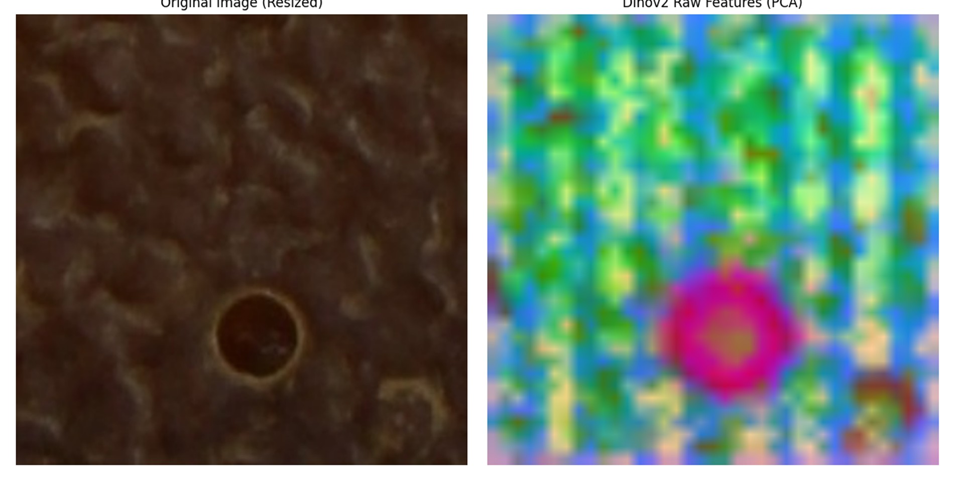
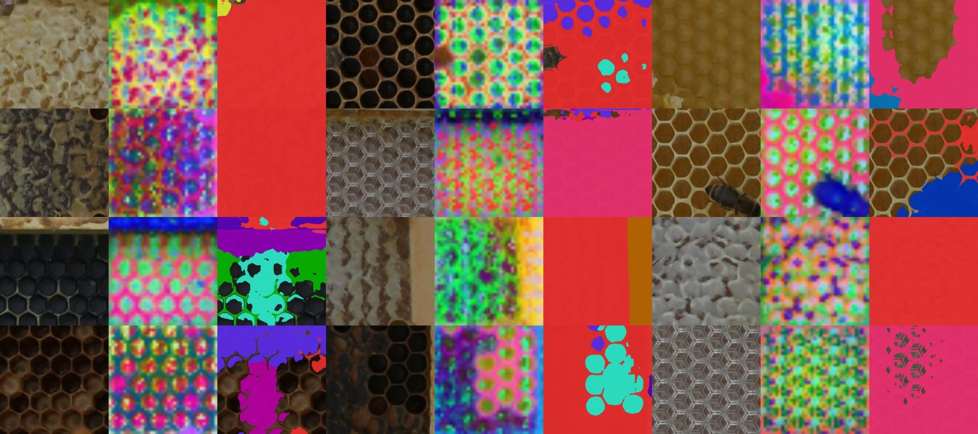
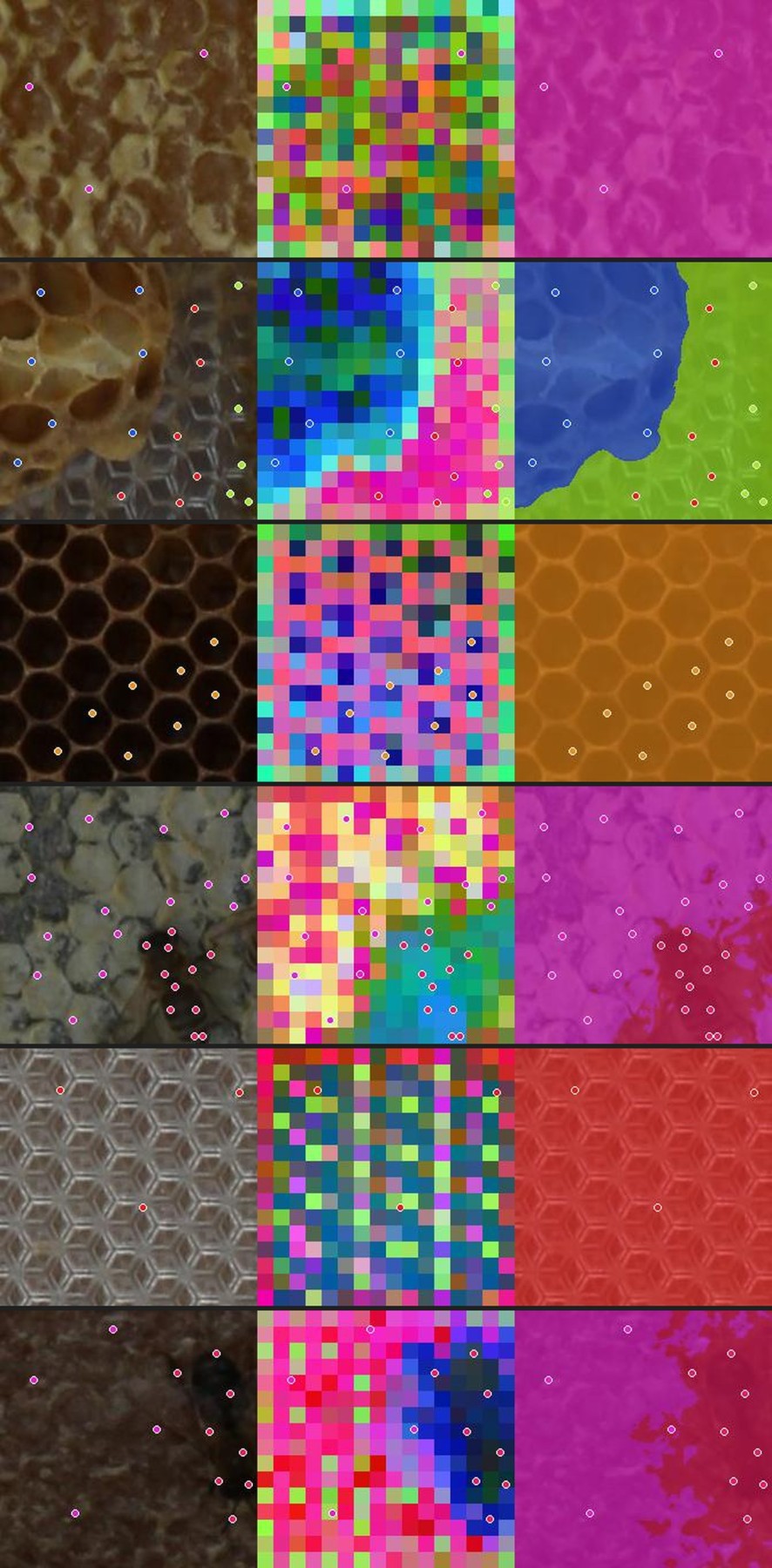
The sparse points supervise a light probe on those embeddings — loss is computed only at the labelled points, everything else ignored. Each panel shows a labelled point and the patch embedding the probe reads there per class. The probe then labels every patch by its embedding and DenseCRF snaps regions to the comb — turning a few points into dense pseudo-masks that train the final model.
A ResUNet (ResNet-101) is distilled on the pseudo-masks, so inference is a single fast forward pass — no DINOv2 or CRF needed. It maps a whole frame into all 24 classes with per-class coverage %.